Demo 4#
This week we will use deep learning to classify land use and land cover (LULC) in the EuroSAT dataset (Helber et al., 2019). The dataset contains of 27,000 labeled Sentinel-2 images over Europe with ten different land use and land cover classes. The paper can be accessed here and the dataset can be accessed here. We will just be using the RGB version so download the EuroSAT_RGB.zip file.
Install packages#
We will use TensorFlow to construct a deep learning model. TensorFlow is a popular open-source machine learning framework developed by Google in 2015. TensorFlow provides a comprehensive ecosystem of tools, libraries, and community resources that support a wide range of tasks, from simple linear regression to complex neural networks. For beginners, TensorFlow offers high-level APIs like Keras, which simplify the process of building and training deep learning models.
Installation instructions are based on the TensorFlow installation page. To install, open up a terminal and run the following commands:
conda create --name tf
Activate the environment
conda activate tf
Install TensorFlow
pip install tensorflow
Install some other useful packages
pip install jupyter scikit-learn matplotlib
Start Jupyter Lab
jupyter lab
Import packages#
# Import packages
import os
import glob
import matplotlib.pyplot as plt
import numpy as np
import itertools
import PIL
from sklearn.metrics import confusion_matrix
# Import Tensorflow packages for building the ResNet-50 model
import tensorflow.python.keras as k
import tensorflow as tf
from tensorflow.keras.layers import Input, Add, Dense, Activation, ZeroPadding2D, BatchNormalization, Flatten, Conv2D, AveragePooling2D, MaxPooling2D, GlobalMaxPooling2D
from tensorflow.keras.initializers import random_uniform, glorot_uniform
from tensorflow.keras.models import Model
from tensorflow.keras.models import load_model
---------------------------------------------------------------------------
ModuleNotFoundError                       Traceback (most recent call last)
Cell In[2], line 2
      1 # Import Tensorflow packages for building the ResNet-50 model
----> 2 import tensorflow.python.keras as k
      3 import tensorflow as tf
      4 from tensorflow.keras.layers import Input, Add, Dense, Activation, ZeroPadding2D, BatchNormalization, Flatten, Conv2D, AveragePooling2D, MaxPooling2D, GlobalMaxPooling2D

ModuleNotFoundError: No module named 'tensorflow'
# Check version
tf.__version__
'2.19.0'
Define training and test data#
We will start by defining the characteristics of our data which we can do by loading one image.
# Open one image file
image = PIL.Image.open('data/EuroSAT_RGB/Highway/Highway_5.jpg')
image

print(image.height, image.width)
64 64
print(image.getextrema())
((40, 231), (65, 222), (79, 217))
It looks like our data are 8-bit (i.e. have values between 0-255). For machine learning, a common practice is to normalize the values to a range between 0 and 1 which we can do by setting rescale to 1/255.
Question 1
Make a figure showing four examples of four different classes (i.e. 16-panel figure)
# Normalize
rescale = 1.0/255
Now we define some other variables. Note that validation_split is the proportion of images that will be held out for testing purposes.
dataset_url = 'data/EuroSAT_RGB/'
batch_size = 32
validation_split = 0.2
TensorFlow has some useful functions for generating training and testing datasets directly from our data directory. The directory structure has to be:
main_directory/
...class_a/
......a_image_1.jpg
......a_image_2.jpg
...class_b/
......b_image_1.jpg
......b_image_2.jpg
datagen = tf.keras.preprocessing.image.ImageDataGenerator(validation_split=validation_split, rescale=rescale)
dataset = tf.keras.preprocessing.image_dataset_from_directory(dataset_url, image_size=(image.height, image.width), batch_size=batch_size)
Found 27000 files belonging to 10 classes.
Once we have these, we can print the class names by running
dataset.class_names
['AnnualCrop',
 'Forest',
 'HerbaceousVegetation',
 'Highway',
 'Industrial',
 'Pasture',
 'PermanentCrop',
 'Residential',
 'River',
 'SeaLake']
# Define training dataset
train_dataset = datagen.flow_from_directory(batch_size=batch_size,
                                           directory=dataset_url,
                                           shuffle=True,
                                           target_size=(image.height, image.width),
                                           subset="training",
                                           class_mode='categorical')
Found 21600 images belonging to 10 classes.
# Define testing dataset
test_dataset = datagen.flow_from_directory(batch_size=batch_size,
                                           directory=dataset_url,
                                           shuffle=True,
                                           target_size=(image.height, image.width),
                                           subset="validation",
                                           class_mode='categorical')
Found 5400 images belonging to 10 classes.
Question 2
What is the distribution of classes in the training dataset? Is there any evidence of class imbalances?
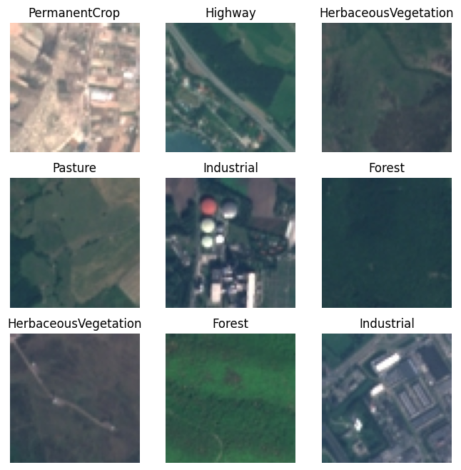
Visualize input datasets#
class_names = dataset.class_names
plt.figure(figsize=(8, 8))
for images, labels in dataset.take(1):
    for i in range(9):
        ax = plt.subplot(3, 3, i + 1)
        plt.imshow(images[i].numpy().astype("uint8"))
        plt.title(class_names[labels[i]])
        plt.axis("off")
2025-04-08 15:19:18.231895: I tensorflow/core/framework/local_rendezvous.cc:407] Local rendezvous is aborting with status: OUT_OF_RANGE: End of sequence
Build ResNet-50 model#
OK now let’s start building a model. We are going to use ResNet-50 which is type of convolutional neural network (CNN) defined by He et al. (2016). ResNet-50 is a variant of the popular ResNet architecture, which stands for “Residual Network.” The “50” in the name refers to the number of layers in the network. ResNet-50 gained significant recognition by winning several visual recognition challenges including the the ImageNet Large Scale Visual Recognition Challenge (ILSVRC). Since then, it has become a foundational model in the field of computer vision, widely used for various applications, including object detection and image segmentation.
def identity_block(X, f, filters, training=True, initializer=random_uniform):
    """
    Implementation of the identity block

    Arguments:
    X -- input tensor of shape (m, n_H_prev, n_W_prev, n_C_prev)
    f -- integer, specifying the shape of the middle CONV's window for the main path
    filters -- python list of integers, defining the number of filters in the CONV layers of the main path
    training -- True: Behave in training mode
                False: Behave in inference mode
    initializer -- to set up the initial weights of a layer. Equals to random uniform initializer

    Returns:
    X -- output of the identity block, tensor of shape (n_H, n_W, n_C)
    """

    # Retrieve Filters
    F1, F2, F3 = filters

    # Save the input value.
    X_shortcut = X
    cache = []
    # First component of main path
    X = Conv2D(filters = F1, kernel_size = 1, strides = (1, 1), padding = 'valid', kernel_initializer = initializer(seed=0))(X)
    X = BatchNormalization(axis = 3)(X, training = training) # Default axis
    X = Activation('relu')(X)

    # Second component of main path (≈3 lines)
    X = Conv2D(filters = F2, kernel_size = (f, f), strides = (1, 1), padding = 'same', kernel_initializer = initializer(seed=0))(X)
    X = BatchNormalization(axis = 3)(X, training = training)
    X = Activation('relu')(X)

    # Third component of main path (≈2 lines)
    X = Conv2D(filters = F3, kernel_size = (1, 1), strides = (1, 1), padding = 'valid', kernel_initializer = initializer(seed=0))(X)
    X = BatchNormalization(axis = 3)(X, training = training)

    # Final step: Add shortcut value to main path, and pass it through a RELU activation (≈2 lines)
    X = Add()([X_shortcut, X])
    X = X = Activation('relu')(X, training = training)

    return X
def convolutional_block(X, f, filters, s = 2, training=True, initializer=glorot_uniform):
    """
    Implementation of the convolutional block

    Arguments:
    X -- input tensor of shape (m, n_H_prev, n_W_prev, n_C_prev)
    f -- integer, specifying the shape of the middle CONV's window for the main path
    filters -- python list of integers, defining the number of filters in the CONV layers of the main path
    s -- Integer, specifying the stride to be used
    training -- True: Behave in training mode
                False: Behave in inference mode
    initializer -- to set up the initial weights of a layer. Equals to Glorot uniform initializer,
                   also called Xavier uniform initializer.

    Returns:
    X -- output of the convolutional block, tensor of shape (n_H, n_W, n_C)
    """

    # Retrieve Filters
    F1, F2, F3 = filters

    # Save the input value
    X_shortcut = X

    ##### MAIN PATH #####

    # First component of main path glorot_uniform(seed=0)
    X = Conv2D(filters = F1, kernel_size = 1, strides = (s, s), padding='valid', kernel_initializer = initializer(seed=0))(X)
    X = BatchNormalization(axis = 3)(X, training=training)
    X = Activation('relu')(X)

    # Second component of main path (≈3 lines)
    X = Conv2D(F2, (f, f), strides = (1, 1), padding = 'same', kernel_initializer = initializer(seed=0))(X)
    X = BatchNormalization(axis = 3)(X, training = training)
    X = Activation('relu')(X)

    # Third component of main path (≈2 lines)
    X = Conv2D(F3, (1, 1), strides = (1, 1), padding = 'valid', kernel_initializer = initializer(seed=0))(X)
    X = BatchNormalization(axis = 3)(X, training = training)

    ##### SHORTCUT PATH #### (≈2 lines)
    X_shortcut = Conv2D(F3, (1, 1), strides = (s, s), padding = 'valid', kernel_initializer = initializer(seed=0))(X_shortcut)
    X_shortcut = BatchNormalization(axis = 3)(X_shortcut, training = training)

    # Final step: Add shortcut value to main path (Use this order [X, X_shortcut]), and pass it through a RELU activation
    X = Add()([X, X_shortcut])
    X = Activation('relu')(X)

    return X
def ResNet50(input_shape = (64, 64, 3), classes = 6):
    """
    Stage-wise implementation of the architecture of the popular ResNet50:
    CONV2D -> BATCHNORM -> RELU -> MAXPOOL -> CONVBLOCK -> IDBLOCK*2 -> CONVBLOCK -> IDBLOCK*3
    -> CONVBLOCK -> IDBLOCK*5 -> CONVBLOCK -> IDBLOCK*2 -> AVGPOOL -> FLATTEN -> DENSE

    Arguments:
    input_shape -- shape of the images of the dataset
    classes -- integer, number of classes

    Returns:
    model -- a Model() instance in Keras
    """

    # Define the input as a tensor with shape input_shape
    X_input = Input(input_shape)


    # Zero-Padding
    X = ZeroPadding2D((3, 3))(X_input)

    # Stage 1
    X = Conv2D(64, (7, 7), strides = (2, 2), kernel_initializer = glorot_uniform(seed=0))(X)
    X = BatchNormalization(axis = 3)(X)
    X = Activation('relu')(X)
    X = MaxPooling2D((3, 3), strides=(2, 2))(X)

    # Stage 2
    X = convolutional_block(X, f = 3, filters = [64, 64, 256], s = 1)
    X = identity_block(X, 3, [64, 64, 256])
    X = identity_block(X, 3, [64, 64, 256])

   # Stage 3 (≈4 lines)
    X = convolutional_block(X, f = 3, filters = [128, 128, 512], s = 2)
    X = identity_block(X, 3, [128, 128, 512])
    X = identity_block(X, 3, [128, 128, 512])
    X = identity_block(X, 3, [128, 128, 512])

    # Stage 4 (≈6 lines)
    X = convolutional_block(X, f = 3, filters = [256, 256, 1024], s = 2)
    X = identity_block(X, 3, [256, 256, 1024])
    X = identity_block(X, 3, [256, 256, 1024])
    X = identity_block(X, 3, [256, 256, 1024])
    X = identity_block(X, 3, [256, 256, 1024])
    X = identity_block(X, 3, [256, 256, 1024])

    # Stage 5 (≈3 lines)
    X = convolutional_block(X, f = 3, filters = [512, 512, 2048], s = 2)
    X = identity_block(X, 3, [512, 512, 2048])
    X = identity_block(X, 3, [512, 512, 2048])

    # AVGPOOL (≈1 line). Use "X = AveragePooling2D(...)(X)"
    X = AveragePooling2D(pool_size = (2, 2), name = 'avg_pool')(X)

    # output layer
    X = Flatten()(X)
    X = Dense(classes, activation='softmax', kernel_initializer = glorot_uniform(seed=0))(X)

    # Create model
    model = Model(inputs = X_input, outputs = X)

    return model
Train model#
After defining the model, we can compile it by specifying an optimizer and loss argument. TensorFlow provides lots of different options. We will use the categorical cross-entropy loss function following Helber et al. (2019). But instead of the SGD optimizer, we will use Adam to speed things up a bit. Definitions of epochs and batch_size can be found on the Keras FAQ page.
# Define model
model = ResNet50(input_shape=(image.height, image.width, 3), classes=10)

# Compile model
model.compile(optimizer='Adam', loss='categorical_crossentropy', metrics=['accuracy'])

# Train
history = model.fit(train_dataset, validation_data=test_dataset, epochs=3, batch_size=32)
Epoch 1/3
675/675 ━━━━━━━━━━━━━━━━━━━━ 405s 587ms/step - accuracy: 0.4468 - loss: 1.8997 - val_accuracy: 0.1020 - val_loss: 2492.8086
Epoch 2/3
675/675 ━━━━━━━━━━━━━━━━━━━━ 412s 609ms/step - accuracy: 0.6619 - loss: 1.0630 - val_accuracy: 0.0926 - val_loss: 1588.7937
Epoch 3/3
675/675 ━━━━━━━━━━━━━━━━━━━━ 408s 604ms/step - accuracy: 0.6740 - loss: 0.9808 - val_accuracy: 0.5917 - val_loss: 1.2601
Note
Now would be a good time to go and get a cup of tea
# Save model
model.save('model/resnet-50-epoch-3-model.keras')
Load model#
model = load_model('model/resnet-50-epoch-3-model.keras')
Confusion matrix#
y_pred = []  # predicted labels
y_true = []  # true labels

# Iterate over the dataset
for i, (image_batch, label_batch) in enumerate(test_dataset):

    # Append true labels
    y_true.append(label_batch)

    # Compute predictions
    preds = model.predict(image_batch, verbose=0)

    # Append predicted labels
    y_pred.append(np.argmax(preds, axis =  1))
    if i==300:
        break

# Convert the true and predicted labels into tensors
correct_labels = tf.concat([item for item in y_true], axis = 0)
correct_labels = np.argmax(correct_labels, axis=1)
predicted_labels = tf.concat([item for item in y_pred], axis = 0)

# Define confusion matrix
cm = confusion_matrix(correct_labels, predicted_labels)
Plot confusion matrix#
plt.figure(figsize=(6, 6))
plt.imshow(cm, interpolation='nearest', cmap='Reds')
plt.colorbar()
tick_marks = np.arange(len(train_dataset.class_indices))
plt.xticks(tick_marks, train_dataset.class_indices, rotation=90)
plt.yticks(tick_marks, train_dataset.class_indices)
thresh = cm.max() / 2.
for i, j in itertools.product(range(cm.shape[0]), range(cm.shape[1])):
    plt.text(j, i, cm[i, j],
        horizontalalignment="center",
        color="white" if cm[i, j] > thresh else "black")

plt.tight_layout()
plt.ylabel('True label')
plt.xlabel('Predicted label')
Text(0.5, -61.902777777777814, 'Predicted label')
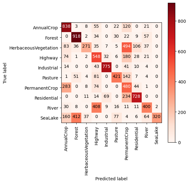
Question 3
a) What is the overall accuracy of the Industrial class?
b) What is the user’s accuracy of the Pasture class?
c) What is the producer’s accuracy of the Residential class?
Concluding statements#
It takes a long time to train the ResNet-50 model on my laptop (600ms/step) so I could only run a few epochs. I’m sure that the model would be a lot more accurate if I could run it over 120 epochs like Helber et al. (2019). As an experiment, I defined a smaller CNN (7 layers). This model only takes 40ms/step on my laptop so I can run it for many more epochs and get a better result. Note that using an NVIDIA T4 GPU in Google Colab, I was able to further improve the speed to 5ms/step.
# Define smaller CNN
model = tf.keras.Sequential([
    Conv2D(32, (3, 3), activation='relu', input_shape=(image.height, image.width, 3)),
    MaxPooling2D((2, 2)),
    Conv2D(64, (3, 3), activation='relu'),
    MaxPooling2D((2, 2)),
    Flatten(),
    Dense(128, activation='relu'),
    Dense(10, activation='softmax')
])

# Compile
model.compile(optimizer='Adam',
              loss='categorical_crossentropy',
              metrics=['accuracy'])

# Fit
history = model.fit(train_dataset, validation_data=test_dataset, epochs=10, batch_size=32)
Epoch 1/10
675/675 ━━━━━━━━━━━━━━━━━━━━ 23s 34ms/step - accuracy: 0.4193 - loss: 1.5379 - val_accuracy: 0.6659 - val_loss: 0.9237
Epoch 2/10
675/675 ━━━━━━━━━━━━━━━━━━━━ 23s 34ms/step - accuracy: 0.6833 - loss: 0.8712 - val_accuracy: 0.7037 - val_loss: 0.7964
Epoch 3/10
675/675 ━━━━━━━━━━━━━━━━━━━━ 23s 35ms/step - accuracy: 0.7480 - loss: 0.6947 - val_accuracy: 0.7585 - val_loss: 0.6613
Epoch 4/10
675/675 ━━━━━━━━━━━━━━━━━━━━ 25s 36ms/step - accuracy: 0.7815 - loss: 0.6000 - val_accuracy: 0.7257 - val_loss: 0.7766
Epoch 5/10
675/675 ━━━━━━━━━━━━━━━━━━━━ 29s 43ms/step - accuracy: 0.8178 - loss: 0.5006 - val_accuracy: 0.7730 - val_loss: 0.6501
Epoch 6/10
675/675 ━━━━━━━━━━━━━━━━━━━━ 27s 39ms/step - accuracy: 0.8428 - loss: 0.4422 - val_accuracy: 0.8085 - val_loss: 0.5378
Epoch 7/10
675/675 ━━━━━━━━━━━━━━━━━━━━ 25s 37ms/step - accuracy: 0.8630 - loss: 0.3850 - val_accuracy: 0.8022 - val_loss: 0.5947
Epoch 8/10
675/675 ━━━━━━━━━━━━━━━━━━━━ 25s 37ms/step - accuracy: 0.8812 - loss: 0.3394 - val_accuracy: 0.7857 - val_loss: 0.6416
Epoch 9/10
675/675 ━━━━━━━━━━━━━━━━━━━━ 25s 37ms/step - accuracy: 0.9012 - loss: 0.2811 - val_accuracy: 0.7950 - val_loss: 0.6320
Epoch 10/10
675/675 ━━━━━━━━━━━━━━━━━━━━ 25s 37ms/step - accuracy: 0.9156 - loss: 0.2390 - val_accuracy: 0.8135 - val_loss: 0.6185
References#
He, K., Zhang, X., Ren, S., & Sun, J. (2016). Deep residual learning for image recognition. In Proceedings of the IEEE conference on computer vision and pattern recognition, 770-778.
Helber, P., Bischke, B., Dengel, A., & Borth, D. (2019). EuroSAT: A novel dataset and deep learning benchmark for land use and land cover classification. IEEE Journal of Selected Topics in Applied Earth Observations and Remote Sensing, 12(7), 2217-2226.
Kshetri, T. (2024). Deep Learning Application for Earth Observation.