EuroSAT activity#
This week we will develop a convolutional network to classify land use and land cover (LULC) in the EuroSAT dataset (Helber et al., 2019). The dataset contains of 27,000 labeled Sentinel-2 images over Europe with ten different land use and land cover classes. The paper can be accessed here and the dataset can be accessed here. We will just be using the RGB version so download the EuroSAT_RGB.zip file.
We should start by activating our TensorFlow environment:
conda activate tf
Open a Jupyter Notebook by running:
jupyter notebook
Import packages#
# Import packages
import os
import glob
import matplotlib.pyplot as plt
import numpy as np
import itertools
import PIL
from sklearn.metrics import confusion_matrix
from tensorflow.keras import layers, preprocessing, models
import tensorflow as tf
---------------------------------------------------------------------------
ModuleNotFoundError                       Traceback (most recent call last)
Cell In[1], line 9
      7 import PIL
      8 from sklearn.metrics import confusion_matrix
----> 9 from tensorflow.keras import layers, preprocessing, models
     10 import tensorflow as tf

ModuleNotFoundError: No module named 'tensorflow'
Explore dataset#
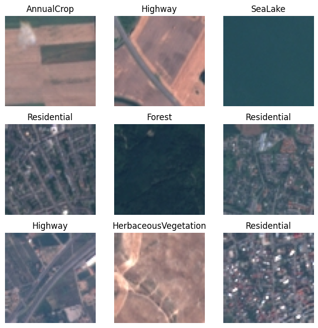
We will start by exploring the dataset by loading one image.
# Open one image file
image = PIL.Image.open('data/EuroSAT_RGB/Highway/Highway_5.jpg')
image

# Print dimensions
print(image.height, image.width)
64 64
# Print min-max values in each band
print(image.getextrema())
((40, 231), (65, 222), (79, 217))
It looks like our data are 8-bit (i.e. have values between 0-255). For machine learning, a common practice is to normalize the values to a range between 0 and 1 which we can do by setting rescale to 1/255.
# Normalize
rescale = 1.0/255
Now we define some other variables. Note that validation_split is the proportion of images that will be held out for testing purposes while the model is training.
dataset_url = 'data/EuroSAT_RGB/'
batch_size = 32
validation_split = 0.2
TensorFlow has some useful functions for generating training and testing datasets directly from our data directory. The directory structure has to be:
main_directory/
...class_a/
......a_image_1.jpg
......a_image_2.jpg
...class_b/
......b_image_1.jpg
......b_image_2.jpg
datagen = preprocessing.image.ImageDataGenerator(validation_split=validation_split, rescale=rescale)
dataset = preprocessing.image_dataset_from_directory(dataset_url, image_size=(image.height, image.width), batch_size=batch_size)
Found 27000 files belonging to 10 classes.
Once we have these, we can print the class names by running
dataset.class_names
['AnnualCrop',
 'Forest',
 'HerbaceousVegetation',
 'Highway',
 'Industrial',
 'Pasture',
 'PermanentCrop',
 'Residential',
 'River',
 'SeaLake']
class_names = dataset.class_names
plt.figure(figsize=(8, 8))
for images, labels in dataset.take(1):
    for i in range(9):
        ax = plt.subplot(3, 3, i + 1)
        plt.imshow(images[i].numpy().astype("uint8"))
        plt.title(class_names[labels[i]])
        plt.axis("off")
2025-10-06 09:20:17.146214: I tensorflow/core/framework/local_rendezvous.cc:407] Local rendezvous is aborting with status: OUT_OF_RANGE: End of sequence
Split into training and testing datasets#
# Define training dataset
train_dataset = datagen.flow_from_directory(batch_size=batch_size,
                                           directory=dataset_url,
                                           shuffle=True,
                                           target_size=(image.height, image.width),
                                           subset="training",
                                           class_mode='categorical')
Found 21600 images belonging to 10 classes.
# Define testing dataset
test_dataset = datagen.flow_from_directory(batch_size=batch_size,
                                           directory=dataset_url,
                                           shuffle=True,
                                           target_size=(image.height, image.width),
                                           subset="validation",
                                           class_mode='categorical')
Found 5400 images belonging to 10 classes.
Build and train model#
Note
May take a few minutes
# Define CNN
model = models.Sequential([
    layers.Input(shape=(image.height, image.width, 3)),
    layers.Conv2D(32, (3, 3), activation='relu'),
    layers.MaxPooling2D((2, 2)),
    layers.Conv2D(64, (3, 3), activation='relu'),
    layers.MaxPooling2D((2, 2)),
    layers.Flatten(),
    layers.Dense(128, activation='relu'),
    layers.Dense(10, activation='softmax')
])

# Compile
model.compile(optimizer='Adam',
              loss='categorical_crossentropy',
              metrics=['accuracy'])

# Fit
history = model.fit(train_dataset, validation_data=test_dataset, epochs=10, batch_size=32)
Epoch 1/10
/opt/miniconda3/envs/tf/lib/python3.11/site-packages/keras/src/trainers/data_adapters/py_dataset_adapter.py:121: UserWarning: Your `PyDataset` class should call `super().__init__(**kwargs)` in its constructor. `**kwargs` can include `workers`, `use_multiprocessing`, `max_queue_size`. Do not pass these arguments to `fit()`, as they will be ignored.
  self._warn_if_super_not_called()
675/675 ━━━━━━━━━━━━━━━━━━━━ 17s 25ms/step - accuracy: 0.4323 - loss: 1.4832 - val_accuracy: 0.6726 - val_loss: 0.9060
Epoch 2/10
675/675 ━━━━━━━━━━━━━━━━━━━━ 17s 26ms/step - accuracy: 0.6987 - loss: 0.8384 - val_accuracy: 0.7537 - val_loss: 0.6880
Epoch 3/10
675/675 ━━━━━━━━━━━━━━━━━━━━ 17s 26ms/step - accuracy: 0.7636 - loss: 0.6447 - val_accuracy: 0.7709 - val_loss: 0.6390
Epoch 4/10
675/675 ━━━━━━━━━━━━━━━━━━━━ 19s 29ms/step - accuracy: 0.8068 - loss: 0.5400 - val_accuracy: 0.7754 - val_loss: 0.6275
Epoch 5/10
675/675 ━━━━━━━━━━━━━━━━━━━━ 21s 32ms/step - accuracy: 0.8247 - loss: 0.4850 - val_accuracy: 0.7887 - val_loss: 0.5870
Epoch 6/10
675/675 ━━━━━━━━━━━━━━━━━━━━ 19s 28ms/step - accuracy: 0.8591 - loss: 0.3913 - val_accuracy: 0.7872 - val_loss: 0.6082
Epoch 7/10
675/675 ━━━━━━━━━━━━━━━━━━━━ 17s 26ms/step - accuracy: 0.8755 - loss: 0.3487 - val_accuracy: 0.8233 - val_loss: 0.5091
Epoch 8/10
675/675 ━━━━━━━━━━━━━━━━━━━━ 19s 28ms/step - accuracy: 0.9004 - loss: 0.2887 - val_accuracy: 0.8178 - val_loss: 0.5720
Epoch 9/10
675/675 ━━━━━━━━━━━━━━━━━━━━ 19s 29ms/step - accuracy: 0.9126 - loss: 0.2476 - val_accuracy: 0.8146 - val_loss: 0.5838
Epoch 10/10
675/675 ━━━━━━━━━━━━━━━━━━━━ 21s 32ms/step - accuracy: 0.9301 - loss: 0.2027 - val_accuracy: 0.7911 - val_loss: 0.6910
Note
Better accuracy could be acheived with a larger model tha is trained for longer. Helber et al. (2021) for example trained a ResNet-50 model for 120 epochs (see Table III) and achieved an overall accuracy of 98.6%.
# Save model
model.save('model/u-net-10-epochs.keras')
Load model#
model = models.load_model('model/u-net-10-epochs.keras')
Confusion matrix#
y_pred = []
y_true = []

# Iterate over the dataset
for i, (image_batch, label_batch) in enumerate(test_dataset):

    # Append true labels
    y_true.append(label_batch)

    # Compute predictions
    preds = model.predict(image_batch, verbose=0)

    # Append predicted labels
    y_pred.append(np.argmax(preds, axis =  1))
    if i==300:
        break

# Convert the true and predicted labels into tensors
correct_labels = tf.concat([item for item in y_true], axis = 0)
correct_labels = np.argmax(correct_labels, axis=1)
predicted_labels = tf.concat([item for item in y_pred], axis = 0)

# Define confusion matrix
cm = confusion_matrix(correct_labels, predicted_labels)
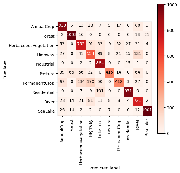
Plot confusion matrix#
plt.figure(figsize=(6, 6))
plt.imshow(cm, interpolation='nearest', cmap='Reds')
plt.colorbar()
tick_marks = np.arange(len(train_dataset.class_indices))
plt.xticks(tick_marks, train_dataset.class_indices, rotation=90)
plt.yticks(tick_marks, train_dataset.class_indices)
thresh = cm.max() / 2.
for i, j in itertools.product(range(cm.shape[0]), range(cm.shape[1])):
    plt.text(j, i, cm[i, j],
        horizontalalignment="center",
        color="white" if cm[i, j] > thresh else "black")

plt.tight_layout()
plt.ylabel('True label')
plt.xlabel('Predicted label')
Text(0.5, -61.902777777777814, 'Predicted label')
Important
Please submit your notebook in .pdf format to Canvas by the deadline as evidence of your work.
References#
Helber, P., Bischke, B., Dengel, A., & Borth, D. (2019). EuroSAT: A novel dataset and deep learning benchmark for land use and land cover classification. IEEE Journal of Selected Topics in Applied Earth Observations and Remote Sensing, 12(7), 2217-2226.
Kshetri, T. (2024). Deep Learning Application for Earth Observation.