Climate data analysis

In this demo, we will be investigating the world’s climate. The data contains gridded monthly air temperature and precipitation for the 1959-2021 time period from the Copernicus Climate Change Service.

xarray

• The best Python package for this task is xarray which introduces labels in the form of dimensions, coordinates, and attributes on top of raw NumPy-like arrays, a bit like Pandas.

• xarray can be used read, write, and analyze any scientific datasets stored in .nc or .hdf format.

• Almost all climate data (and some remote sensing data) are stored in these formats.

# Import package
import xarray as xr
import numpy as np
import matplotlib.pyplot as plt
from mpl_toolkits.axes_grid1 import make_axes_locatable

# Read data
xds = xr.open_dataset('data/world_climate.nc')

Basic information about Dataset

type(xds)

xarray.core.dataset.Dataset

xds.dims

FrozenMappingWarningOnValuesAccess({'longitude': 1440, 'latitude': 721, 'time': 756})

xds.coords

Coordinates:
  * longitude  (longitude) float32 6kB 0.0 0.25 0.5 0.75 ... 359.2 359.5 359.8
  * latitude   (latitude) float32 3kB 90.0 89.75 89.5 ... -89.5 -89.75 -90.0
  * time       (time) datetime64[ns] 6kB 1959-01-01 1959-02-01 ... 2021-12-01

All information can be printed using the keys() function.

xds.keys

<bound method Mapping.keys of <xarray.Dataset> Size: 13GB
Dimensions:    (longitude: 1440, latitude: 721, time: 756)
Coordinates:
  * longitude  (longitude) float32 6kB 0.0 0.25 0.5 0.75 ... 359.2 359.5 359.8
  * latitude   (latitude) float32 3kB 90.0 89.75 89.5 ... -89.5 -89.75 -90.0
  * time       (time) datetime64[ns] 6kB 1959-01-01 1959-02-01 ... 2021-12-01
Data variables:
    t2m        (time, latitude, longitude) float64 6GB ...
    mtpr       (time, latitude, longitude) float64 6GB ...
Attributes:
    Conventions:  CF-1.6
    history:      2023-01-28 21:51:01 GMT by grib_to_netcdf-2.25.1: /opt/ecmw...>

Note

t2m stands for 2 m above the surface, the standard height used by temperature sensors. It is a common metric used in climatology but note that it is different from the surface temperature which would be the temperature of the ground surface.

Since we are using an interactive notebook, a more convenient way of finding information about our dataset is to just execute the variable name.

xds

<xarray.Dataset> Size: 13GB
Dimensions:    (longitude: 1440, latitude: 721, time: 756)
Coordinates:
  * longitude  (longitude) float32 6kB 0.0 0.25 0.5 0.75 ... 359.2 359.5 359.8
  * latitude   (latitude) float32 3kB 90.0 89.75 89.5 ... -89.5 -89.75 -90.0
  * time       (time) datetime64[ns] 6kB 1959-01-01 1959-02-01 ... 2021-12-01
Data variables:
    t2m        (time, latitude, longitude) float64 6GB ...
    mtpr       (time, latitude, longitude) float64 6GB ...
Attributes:
    Conventions:  CF-1.6
    history:      2023-01-28 21:51:01 GMT by grib_to_netcdf-2.25.1: /opt/ecmw...

xarray.Dataset

• Dimensions:
  • longitude: 1440
  • latitude: 721
  • time: 756
• Coordinates: (3)
  • longitude
    (longitude)
    float32
    0.0 0.25 0.5 ... 359.2 359.5 359.8

    units :

    degrees_east

    long_name :

    longitude

    array([0.0000e+00, 2.5000e-01, 5.0000e-01, ..., 3.5925e+02, 3.5950e+02,
           3.5975e+02], shape=(1440,), dtype=float32)

  • latitude
    (latitude)
    float32
    90.0 89.75 89.5 ... -89.75 -90.0

    units :

    degrees_north

    long_name :

    latitude

    array([ 90.  ,  89.75,  89.5 , ..., -89.5 , -89.75, -90.  ],
          shape=(721,), dtype=float32)

  • time
    (time)
    datetime64[ns]
    1959-01-01 ... 2021-12-01

    long_name :

    time

    array(['1959-01-01T00:00:00.000000000', '1959-02-01T00:00:00.000000000',
           '1959-03-01T00:00:00.000000000', ..., '2021-10-01T00:00:00.000000000',
           '2021-11-01T00:00:00.000000000', '2021-12-01T00:00:00.000000000'],
          shape=(756,), dtype='datetime64[ns]')

• Data variables: (2)
  • t2m
    (time, latitude, longitude)
    float64
    ...

    units :

    K

    long_name :

    2 metre temperature

    [784909440 values with dtype=float64]

  • mtpr
    (time, latitude, longitude)
    float64
    ...

    units :

    kg m**-2 s**-1

    long_name :

    Mean total precipitation rate

    [784909440 values with dtype=float64]

• Indexes: (3)
  • longitude
    PandasIndex

    PandasIndex(Index([   0.0,   0.25,    0.5,   0.75,    1.0,   1.25,    1.5,   1.75,    2.0,
             2.25,
           ...
            357.5, 357.75,  358.0, 358.25,  358.5, 358.75,  359.0, 359.25,  359.5,
           359.75],
          dtype='float32', name='longitude', length=1440))

  • latitude
    PandasIndex

    PandasIndex(Index([  90.0,  89.75,   89.5,  89.25,   89.0,  88.75,   88.5,  88.25,   88.0,
            87.75,
           ...
           -87.75,  -88.0, -88.25,  -88.5, -88.75,  -89.0, -89.25,  -89.5, -89.75,
            -90.0],
          dtype='float32', name='latitude', length=721))

  • time
    PandasIndex

    PandasIndex(DatetimeIndex(['1959-01-01', '1959-02-01', '1959-03-01', '1959-04-01',
                   '1959-05-01', '1959-06-01', '1959-07-01', '1959-08-01',
                   '1959-09-01', '1959-10-01',
                   ...
                   '2021-03-01', '2021-04-01', '2021-05-01', '2021-06-01',
                   '2021-07-01', '2021-08-01', '2021-09-01', '2021-10-01',
                   '2021-11-01', '2021-12-01'],
                  dtype='datetime64[ns]', name='time', length=756, freq=None))

• Attributes: (2)

  Conventions :

  CF-1.6

  history :

  2023-01-28 21:51:01 GMT by grib_to_netcdf-2.25.1: /opt/ecmwf/mars-client/bin/grib_to_netcdf.bin -S param -o /cache/data2/adaptor.mars.internal-1674942629.839177-10303-1-835fc652-769e-4b52-a99b-06011f72baf8.nc /cache/tmp/835fc652-769e-4b52-a99b-06011f72baf8-adaptor.mars.internal-1674942395.056822-10303-1-tmp.grib

Basic information about DataArray

type(xds['latitude'])

xarray.core.dataarray.DataArray

xds['latitude']

<xarray.DataArray 'latitude' (latitude: 721)> Size: 3kB
array([ 90.  ,  89.75,  89.5 , ..., -89.5 , -89.75, -90.  ],
      shape=(721,), dtype=float32)
Coordinates:
  * latitude  (latitude) float32 3kB 90.0 89.75 89.5 ... -89.5 -89.75 -90.0
Attributes:
    units:      degrees_north
    long_name:  latitude

xarray.DataArray

'latitude'

• latitude: 721

• 90.0 89.75 89.5 89.25 89.0 88.75 ... -89.0 -89.25 -89.5 -89.75 -90.0

  array([ 90.  ,  89.75,  89.5 , ..., -89.5 , -89.75, -90.  ],
        shape=(721,), dtype=float32)

• Coordinates: (1)
  • latitude
    (latitude)
    float32
    90.0 89.75 89.5 ... -89.75 -90.0

    units :

    degrees_north

    long_name :

    latitude

    array([ 90.  ,  89.75,  89.5 , ..., -89.5 , -89.75, -90.  ],
          shape=(721,), dtype=float32)

• Indexes: (1)
  • latitude
    PandasIndex

    PandasIndex(Index([  90.0,  89.75,   89.5,  89.25,   89.0,  88.75,   88.5,  88.25,   88.0,
            87.75,
           ...
           -87.75,  -88.0, -88.25,  -88.5, -88.75,  -89.0, -89.25,  -89.5, -89.75,
            -90.0],
          dtype='float32', name='latitude', length=721))

• Attributes: (2)

  units :

  degrees_north

  long_name :

  latitude

Print as a NumPy array

type(xds['latitude'].values)

numpy.ndarray

First item in array

xds['latitude'].values[0]

np.float32(90.0)

Last item in array

xds['latitude'].values[-1]

np.float32(-90.0)

Shape of DataArray

xds['latitude'].values.shape

(721,)

Time

type(xds['time'].values[0])

numpy.datetime64

period = xds['time'].values[-1] - xds['time'].values[0]
period

np.timedelta64(1985472000000000000,'ns')

period.astype('timedelta64[Y]')

np.timedelta64(62,'Y')

Convert to integer

period.astype('timedelta64[Y]').astype(int)

np.int64(62)

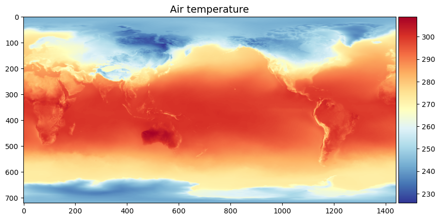
Plot

fig, ax = plt.subplots(figsize=(10,6))

im1 = ax.imshow(xds['t2m'][0,:,:], cmap='RdYlBu_r')

ax.set_title("Air temperature", fontsize=14)
divider = make_axes_locatable(ax)
cax = divider.append_axes('right', size='5%', pad=0.05)
fig.colorbar(im1, cax=cax, orientation='vertical')

<matplotlib.colorbar.Colorbar at 0x15e363110>

Stats

Compute mean air temperature for entire period

temp = xds['t2m']
mean_temp = temp.mean(['time'])
mean_temp

<xarray.DataArray 't2m' (latitude: 721, longitude: 1440)> Size: 8MB
array([[258.49005406, 258.49005406, 258.49005406, ..., 258.49005406,
        258.49005406, 258.49005406],
       [258.49639085, 258.49655877, 258.49666606, ..., 258.49590574,
        258.49609931, 258.49620893],
       [258.54803436, 258.54841452, 258.54879001, ..., 258.54686356,
        258.54714576, 258.54754691],
       ...,
       [228.08867964, 228.0895729 , 228.09131278, ..., 228.08614213,
        228.08758348, 228.08856303],
       [227.98272217, 227.98401892, 227.98524336, ..., 227.98061613,
        227.98129249, 227.98197351],
       [227.51711896, 227.51711896, 227.51711896, ..., 227.51711896,
        227.51711896, 227.51711896]], shape=(721, 1440))
Coordinates:
  * longitude  (longitude) float32 6kB 0.0 0.25 0.5 0.75 ... 359.2 359.5 359.8
  * latitude   (latitude) float32 3kB 90.0 89.75 89.5 ... -89.5 -89.75 -90.0

xarray.DataArray

't2m'

• latitude: 721
• longitude: 1440

• 258.5 258.5 258.5 258.5 258.5 258.5 ... 227.5 227.5 227.5 227.5 227.5

  array([[258.49005406, 258.49005406, 258.49005406, ..., 258.49005406,
          258.49005406, 258.49005406],
         [258.49639085, 258.49655877, 258.49666606, ..., 258.49590574,
          258.49609931, 258.49620893],
         [258.54803436, 258.54841452, 258.54879001, ..., 258.54686356,
          258.54714576, 258.54754691],
         ...,
         [228.08867964, 228.0895729 , 228.09131278, ..., 228.08614213,
          228.08758348, 228.08856303],
         [227.98272217, 227.98401892, 227.98524336, ..., 227.98061613,
          227.98129249, 227.98197351],
         [227.51711896, 227.51711896, 227.51711896, ..., 227.51711896,
          227.51711896, 227.51711896]], shape=(721, 1440))

• Coordinates: (2)
  • longitude
    (longitude)
    float32
    0.0 0.25 0.5 ... 359.2 359.5 359.8

    units :

    degrees_east

    long_name :

    longitude

    array([0.0000e+00, 2.5000e-01, 5.0000e-01, ..., 3.5925e+02, 3.5950e+02,
           3.5975e+02], shape=(1440,), dtype=float32)

  • latitude
    (latitude)
    float32
    90.0 89.75 89.5 ... -89.75 -90.0

    units :

    degrees_north

    long_name :

    latitude

    array([ 90.  ,  89.75,  89.5 , ..., -89.5 , -89.75, -90.  ],
          shape=(721,), dtype=float32)

• Indexes: (2)
  • longitude
    PandasIndex

    PandasIndex(Index([   0.0,   0.25,    0.5,   0.75,    1.0,   1.25,    1.5,   1.75,    2.0,
             2.25,
           ...
            357.5, 357.75,  358.0, 358.25,  358.5, 358.75,  359.0, 359.25,  359.5,
           359.75],
          dtype='float32', name='longitude', length=1440))

  • latitude
    PandasIndex

    PandasIndex(Index([  90.0,  89.75,   89.5,  89.25,   89.0,  88.75,   88.5,  88.25,   88.0,
            87.75,
           ...
           -87.75,  -88.0, -88.25,  -88.5, -88.75,  -89.0, -89.25,  -89.5, -89.75,
            -90.0],
          dtype='float32', name='latitude', length=721))

• Attributes: (0)

mean_temp.shape

(721, 1440)

mean_temp[300, 100]

<xarray.DataArray 't2m' ()> Size: 8B
array(297.00346626)
Coordinates:
    longitude  float32 4B 25.0
    latitude   float32 4B 15.0

xarray.DataArray

't2m'

• 297.0

  array(297.00346626)

• Coordinates: (2)
  • longitude
    ()
    float32
    25.0

    units :

    degrees_east

    long_name :

    longitude

    array(25., dtype=float32)

  • latitude
    ()
    float32
    15.0

    units :

    degrees_north

    long_name :

    latitude

    array(15., dtype=float32)

• Indexes: (0)
• Attributes: (0)

# Plot
fig, ax = plt.subplots(figsize=(10,6))

im1 = ax.imshow(xds['t2m'][0,:,:], cmap='RdYlBu_r')
ax.scatter(100, 300, s=100, c='k')

ax.set_title("Air temperature", fontsize=14)
divider = make_axes_locatable(ax)
cax = divider.append_axes('right', size='5%', pad=0.05)
fig.colorbar(im1, cax=cax, orientation='vertical')

<matplotlib.colorbar.Colorbar at 0x1603ff830>

Indexing multi-dimensional datasets

Since our xarray dataset is aware of the latitude and longitude coordinates, we can index values conveniently.

t = xds['t2m'].sel(latitude=27.7, longitude=85.3, method='nearest')
print('The mean annual air temperature in Kathmandu is %.2f F' %((t.mean('time').values - 273.15) * 9/5 + 32))

The mean annual air temperature in Kathmandu is 62.49 F

Convert to Pandas DataFrame

t.to_dataframe()

	longitude	latitude	t2m
time
1959-01-01	85.25	27.75	282.517155
1959-02-01	85.25	27.75	283.446361
1959-03-01	85.25	27.75	288.469712
1959-04-01	85.25	27.75	293.018762
1959-05-01	85.25	27.75	294.681458
...	...	...	...
2021-08-01	85.25	27.75	295.180443
2021-09-01	85.25	27.75	294.954754
2021-10-01	85.25	27.75	292.877707
2021-11-01	85.25	27.75	287.104996
2021-12-01	85.25	27.75	283.973557

756 rows × 3 columns

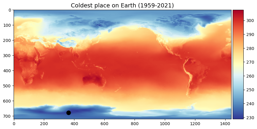
Where is the coldest place on Earth (1959-2021)?

To find the coldest place on Earth we have to find the grid cell with the lowest temperature. The argmin() function returns the indices of the minimum values of an array.

min_value = mean_temp.argmin()
print(min_value)

<xarray.DataArray 't2m' ()> Size: 8B
array(978122)

Perhaps unexpectedly, argmin() returns a single number instead of a row/column pair. We can use NumPy’s unravel_index() to convert this 1D index to 2D coordinates. It just needs to know the shape of our original 2D DataArray.

low_idx = np.unravel_index(min_value, mean_temp.shape)
print(low_idx)

(np.int64(679), np.int64(362))

cold = mean_temp[low_idx[0], low_idx[1]].values
print('Coldest place on Earth is %.2f F' % ((cold - 273.15) * 9/5 + 32))

Coldest place on Earth is -64.64 F

fig, ax1 = plt.subplots(figsize=(10,6))

im1 = ax1.imshow(xds['t2m'][1,:,:], cmap='RdYlBu_r')

ax1.set_title("Coldest place on Earth (1959-2021)", fontsize=14)
ax1.scatter(low_idx[1], low_idx[0], s=100, color='k')

divider = make_axes_locatable(ax1)
cax = divider.append_axes('right', size='5%', pad=0.05)
fig.colorbar(im1, cax=cax, orientation='vertical')

<matplotlib.colorbar.Colorbar at 0x1604b19d0>

Which was the hottest month on Earth (1959-2021)?

To find the hottest month on Earth, we need to preserve the time dimension of our data. Instead we need average over the latitude and longitude dimensions.

hot = xds['t2m'].mean(['longitude','latitude'])

hot['time'][hot.argmax()].values

np.datetime64('2019-07-01T00:00:00.000000000')

Which was July 2019!!

Which was the hottest year on Earth (1959-2021)?

There are a couple of ways to find the hottest year. The first is to use the groupby function.

temp_yearly = xds['t2m'].groupby('time.year').mean()

hot = temp_yearly.mean(['longitude','latitude'])
hot['year'][hot.argmax()].values

array(2016)

Note

Since we grouped by year, the time interval dimension was renamed to year.

Alternatively, we could use the resample function.

temp_yearly = xds['t2m'].resample(time="YE").mean()

hot = temp_yearly.mean(['longitude','latitude'])
hot['time'][hot.argmax()].values

np.datetime64('2016-12-31T00:00:00.000000000')