Vector data analysis#
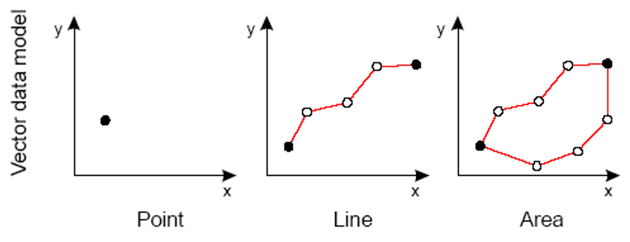
The vector data model represents space as a series of discrete entities such as such as borders, buildings, streets, and roads. There are three different types of vector data: points, lines and polygons. Online mapping applications, such as Google Maps and OpenStreetMap, use this format to display data.
The Python library GeoPandas provides somes great tools for working with vector data. As the name suggests, GeoPandas extends the popular data science library Pandas by adding support for geospatial data. The core data structure in GeoPandas is the GeoDataFrame. The key difference between the two is that a GeoDataFrame can store geometry data and perform spatial operations.
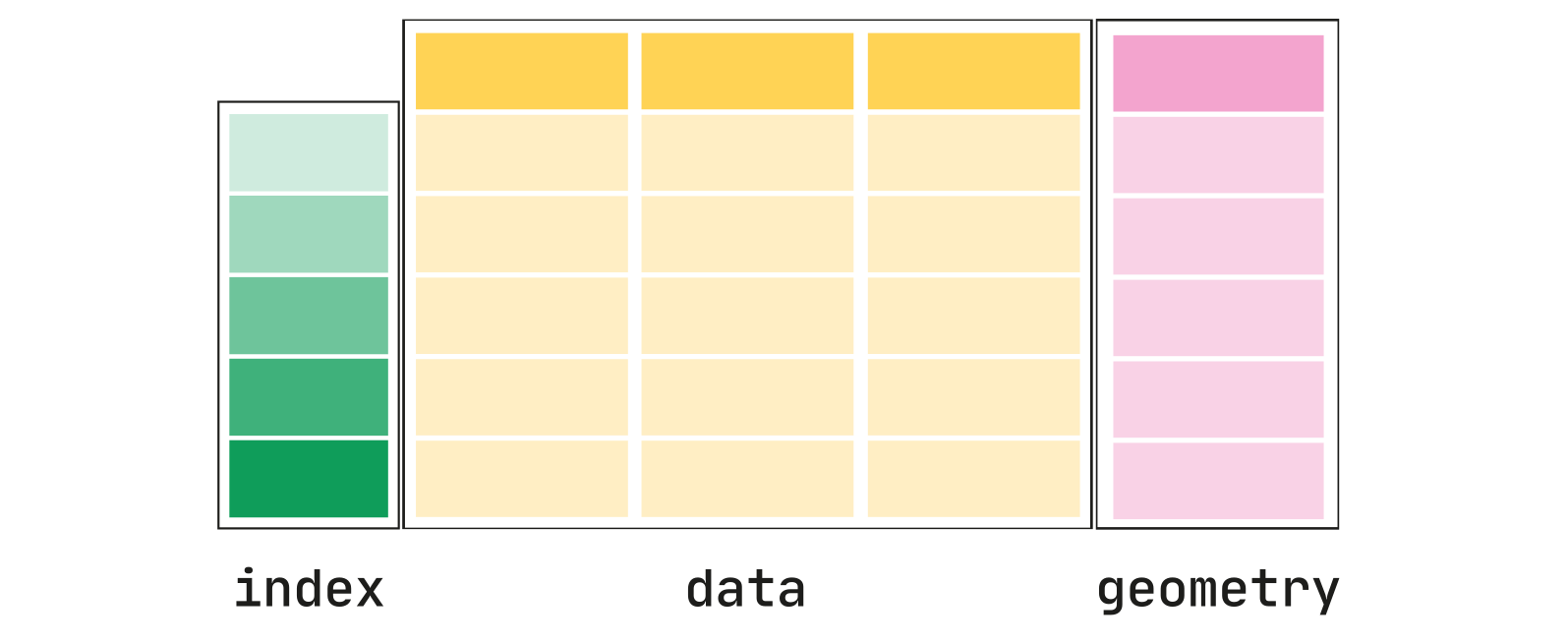
The geometry column can contain any geometry type (e.g. points, lines, polygons) or even a mixture.
Reading files#
Assuming we have a file containing both data and geometry (e.g. GeoPackage, GeoJSON, Shapefile), we can read it using read_file, which automatically detects the filetype and creates a GeoDataFrame. In the this demo, we will be working with two shapefiles containing 1) cities and towns (as points), and 2) counties (as polygons) in Oregon.
import os
os.environ['USE_PYGEOS'] = '0'
import geopandas as gpd

cities = gpd.read_file('data/oregon_cities.shp')
cities.head()
| name | lat | lon | geometry | |
|---|---|---|---|---|
| 0 | Adair Village city | 44.67 | -123.22 | POINT (-123.22 44.67) |
| 1 | Adams | 45.77 | -118.56 | POINT (-118.56 45.77) |
| 2 | Adrian | 43.74 | -117.07 | POINT (-117.07 43.74) |
| 3 | Albany | 44.63 | -123.10 | POINT (-123.1 44.63) |
| 4 | Aloha | 45.49 | -122.87 | POINT (-122.87 45.49) |
DataFrame properties#
We can analyze our GeoDataFrame using standard Pandas functions.
# Data types of each column
cities.dtypes
name          object
lat          float64
lon          float64
geometry    geometry
dtype: object
# Number of rows and columns
cities.shape
(377, 4)
# Name of columns
cities.columns
Index(['name', 'lat', 'lon', 'geometry'], dtype='object')
Indexing#
We can select specific columns based on the column values. The basic syntax is dataframe[value], where value can be a single column name, or a list of column names.
# List the city names
cities['name']
0      Adair Village city
1                   Adams
2                  Adrian
3                  Albany
4                   Aloha
              ...
372          Wood Village
373              Woodburn
374               Yachats
375               Yamhill
376              Yoncalla
Name: name, Length: 377, dtype: object
# List the latitudes and longitudes
cities[['lat','lon']]
| lat | lon | |
|---|---|---|
| 0 | 44.67 | -123.22 |
| 1 | 45.77 | -118.56 |
| 2 | 43.74 | -117.07 |
| 3 | 44.63 | -123.10 |
| 4 | 45.49 | -122.87 |
| ... | ... | ... |
| 372 | 45.54 | -122.42 |
| 373 | 45.15 | -122.86 |
| 374 | 44.31 | -124.10 |
| 375 | 45.34 | -123.19 |
| 376 | 43.60 | -123.29 |
377 rows × 2 columns
We can select specific rows using the .iloc method.
# Second row
cities.iloc[1]
name                        Adams
lat                         45.77
lon                       -118.56
geometry    POINT (-118.56 45.77)
Name: 1, dtype: object
# Sixth to tenth rows
cities.iloc[5:10]
| name | lat | lon | geometry | |
|---|---|---|---|---|
| 5 | Alpine | 44.33 | -123.36 | POINT (-123.36 44.33) |
| 6 | Alsea | 44.38 | -123.60 | POINT (-123.6 44.38) |
| 7 | Altamont | 42.20 | -121.72 | POINT (-121.72 42.2) |
| 8 | Amity | 45.12 | -123.20 | POINT (-123.2 45.12) |
| 9 | Annex | 44.23 | -116.99 | POINT (-116.99 44.23) |
Masking#
We can sample of our DataFrame based on specific values by producing a Boolean mask (i.e. a list of values equal to True or False). To find cities that are East of -117.5 degrees longitude, we could write:
mask = cities['lon'] > -117.5
cities[mask]
| name | lat | lon | geometry | |
|---|---|---|---|---|
| 2 | Adrian | 43.74 | -117.07 | POINT (-117.07 43.74) |
| 9 | Annex | 44.23 | -116.99 | POINT (-116.99 44.23) |
| 97 | Enterprise | 45.43 | -117.28 | POINT (-117.28 45.43) |
| 134 | Halfway | 44.88 | -117.11 | POINT (-117.11 44.88) |
| 150 | Huntington | 44.35 | -117.27 | POINT (-117.27 44.35) |
| 164 | Jordan Valley | 42.98 | -117.06 | POINT (-117.06 42.98) |
| 165 | Joseph | 45.35 | -117.23 | POINT (-117.23 45.35) |
| 190 | Lostine | 45.49 | -117.43 | POINT (-117.43 45.49) |
| 238 | Nyssa | 43.88 | -117.00 | POINT (-117 43.88) |
| 247 | Ontario | 44.03 | -116.98 | POINT (-116.98 44.03) |
| 274 | Richland | 44.77 | -117.17 | POINT (-117.17 44.77) |
| 345 | Vale | 43.98 | -117.24 | POINT (-117.24 43.98) |
| 350 | Wallowa Lake | 45.30 | -117.21 | POINT (-117.21 45.3) |
It’s more concise to just add the Boolean mask between square brackets. Here we find a specific city.
cities[cities['name'] == 'Eugene']
| name | lat | lon | geometry | |
|---|---|---|---|---|
| 100 | Eugene | 44.06 | -123.12 | POINT (-123.12 44.06) |
Or cities that contain a z in their name.
cities[cities['name'].str.contains('z')]
| name | lat | lon | geometry | |
|---|---|---|---|---|
| 34 | Bonanza | 42.20 | -121.41 | POINT (-121.41 42.2) |
| 168 | Keizer | 45.00 | -123.02 | POINT (-123.02 45) |
| 195 | Manzanita | 45.72 | -123.94 | POINT (-123.94 45.72) |
| 206 | Metzger | 45.45 | -122.76 | POINT (-122.76 45.45) |
| 302 | Siletz | 44.72 | -123.92 | POINT (-123.92 44.72) |
Descriptive statistics#
Pandas provides basic functions to calculate descriptive statistics.
# Minimum latitude value
cities['lat'].min()
np.float64(42.0)
# Mean longitude value
cities['lon'].mean()
np.float64(-122.02392572944296)
A full list of descriptive statistics (including some very useful ones such as sum and count) can be found here.
Sometimes we want to know which row contains the specific value which we can do using idxmax/idxmin.
cities['lat'].idxmin()
232
cities.iloc[232]
name           New Pine Creek
lat                      42.0
lon                    -120.3
geometry    POINT (-120.3 42)
Name: 232, dtype: object
Sorting#
We can sort DataFrames using the sort_values function. This function takes two arguments, by and ascending which determine which column and which order we would like to sort by.
# Find the ten most northerly cities in Oregon
cities.sort_values(by='lat', ascending=False).head(10)
| name | lat | lon | geometry | |
|---|---|---|---|---|
| 13 | Astoria | 46.19 | -123.81 | POINT (-123.81 46.19) |
| 354 | Warrenton | 46.17 | -123.92 | POINT (-123.92 46.17) |
| 159 | Jeffers Gardens | 46.15 | -123.85 | POINT (-123.85 46.15) |
| 363 | Westport | 46.13 | -123.37 | POINT (-123.37 46.13) |
| 60 | Clatskanie | 46.10 | -123.21 | POINT (-123.21 46.1) |
| 269 | Rainier | 46.09 | -122.95 | POINT (-122.95 46.09) |
| 265 | Prescott | 46.05 | -122.89 | POINT (-122.89 46.05) |
| 116 | Gearhart | 46.03 | -123.92 | POINT (-123.92 46.03) |
| 293 | Seaside | 45.99 | -123.92 | POINT (-123.92 45.99) |
| 341 | Umapine | 45.98 | -118.50 | POINT (-118.5 45.98) |
An alternative way of doing this would be to use the nlargest/nsmallest functions.
cities.nlargest(n=10, columns='lat')
| name | lat | lon | geometry | |
|---|---|---|---|---|
| 13 | Astoria | 46.19 | -123.81 | POINT (-123.81 46.19) |
| 354 | Warrenton | 46.17 | -123.92 | POINT (-123.92 46.17) |
| 159 | Jeffers Gardens | 46.15 | -123.85 | POINT (-123.85 46.15) |
| 363 | Westport | 46.13 | -123.37 | POINT (-123.37 46.13) |
| 60 | Clatskanie | 46.10 | -123.21 | POINT (-123.21 46.1) |
| 269 | Rainier | 46.09 | -122.95 | POINT (-122.95 46.09) |
| 265 | Prescott | 46.05 | -122.89 | POINT (-122.89 46.05) |
| 116 | Gearhart | 46.03 | -123.92 | POINT (-123.92 46.03) |
| 293 | Seaside | 45.99 | -123.92 | POINT (-123.92 45.99) |
| 341 | Umapine | 45.98 | -118.50 | POINT (-118.5 45.98) |
Geometric properties#
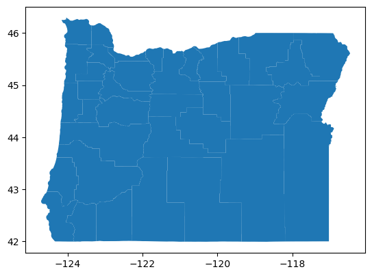
The special thing about a GeoDataFrame is that it contains a geometry column. We can therefore apply spatial methods to these data. To demonstrate we will use our Oregon county shapefile.
# Read shapefile
counties = gpd.read_file('data/orcntypoly.shp')
counties.plot()
<Axes: >
Projections#
GeoDataFrames have their own CRS which can be accessed using the crs method. The CRS tells GeoPandas where the coordinates of the geometries are located on the Earth’s surface.
counties.crs
<Geographic 2D CRS: EPSG:4269>
Name: NAD83
Axis Info [ellipsoidal]:
- Lat[north]: Geodetic latitude (degree)
- Lon[east]: Geodetic longitude (degree)
Area of Use:
- name: North America - onshore and offshore: Canada - Alberta; British Columbia; Manitoba; New Brunswick; Newfoundland and Labrador; Northwest Territories; Nova Scotia; Nunavut; Ontario; Prince Edward Island; Quebec; Saskatchewan; Yukon. Puerto Rico. United States (USA) - Alabama; Alaska; Arizona; Arkansas; California; Colorado; Connecticut; Delaware; Florida; Georgia; Hawaii; Idaho; Illinois; Indiana; Iowa; Kansas; Kentucky; Louisiana; Maine; Maryland; Massachusetts; Michigan; Minnesota; Mississippi; Missouri; Montana; Nebraska; Nevada; New Hampshire; New Jersey; New Mexico; New York; North Carolina; North Dakota; Ohio; Oklahoma; Oregon; Pennsylvania; Rhode Island; South Carolina; South Dakota; Tennessee; Texas; Utah; Vermont; Virginia; Washington; West Virginia; Wisconsin; Wyoming. US Virgin Islands. British Virgin Islands.
- bounds: (167.65, 14.92, -40.73, 86.45)
Datum: North American Datum 1983
- Ellipsoid: GRS 1980
- Prime Meridian: Greenwich
counties['area'] = counties['geometry'].area
counties.head()
/var/folders/6m/lbbbs2n90xq6lk5v5902brkc0000gq/T/ipykernel_43972/945249447.py:1: UserWarning: Geometry is in a geographic CRS. Results from 'area' are likely incorrect. Use 'GeoSeries.to_crs()' to re-project geometries to a projected CRS before this operation.

  counties['area'] = counties['geometry'].area
| county | geometry | area | |
|---|---|---|---|
| 0 | Josephine County | POLYGON ((-123.22962 42.70261, -123.2296 42.69... | 0.464440 |
| 1 | Curry County | POLYGON ((-123.81155 42.78884, -123.81155 42.7... | 0.565393 |
| 2 | Jackson County | POLYGON ((-122.28273 42.9965, -122.28273 42.99... | 0.793753 |
| 3 | Coos County | POLYGON ((-123.81155 42.78884, -123.81638 42.7... | 0.518952 |
| 4 | Klamath County | POLYGON ((-121.33297 43.61665, -121.33296 43.6... | 1.746031 |
We produced an area column but we were warned that our areas are likely to be incorrect. The reason is because the units of the county boundaries are in degrees (i.e. angular units). Since degrees vary in actual ground distance depending on location (for example, 1° longitude is ~111 km at the equator but almost 0 km at the poles), areas calculated directly from lat/lon values are meaningless.

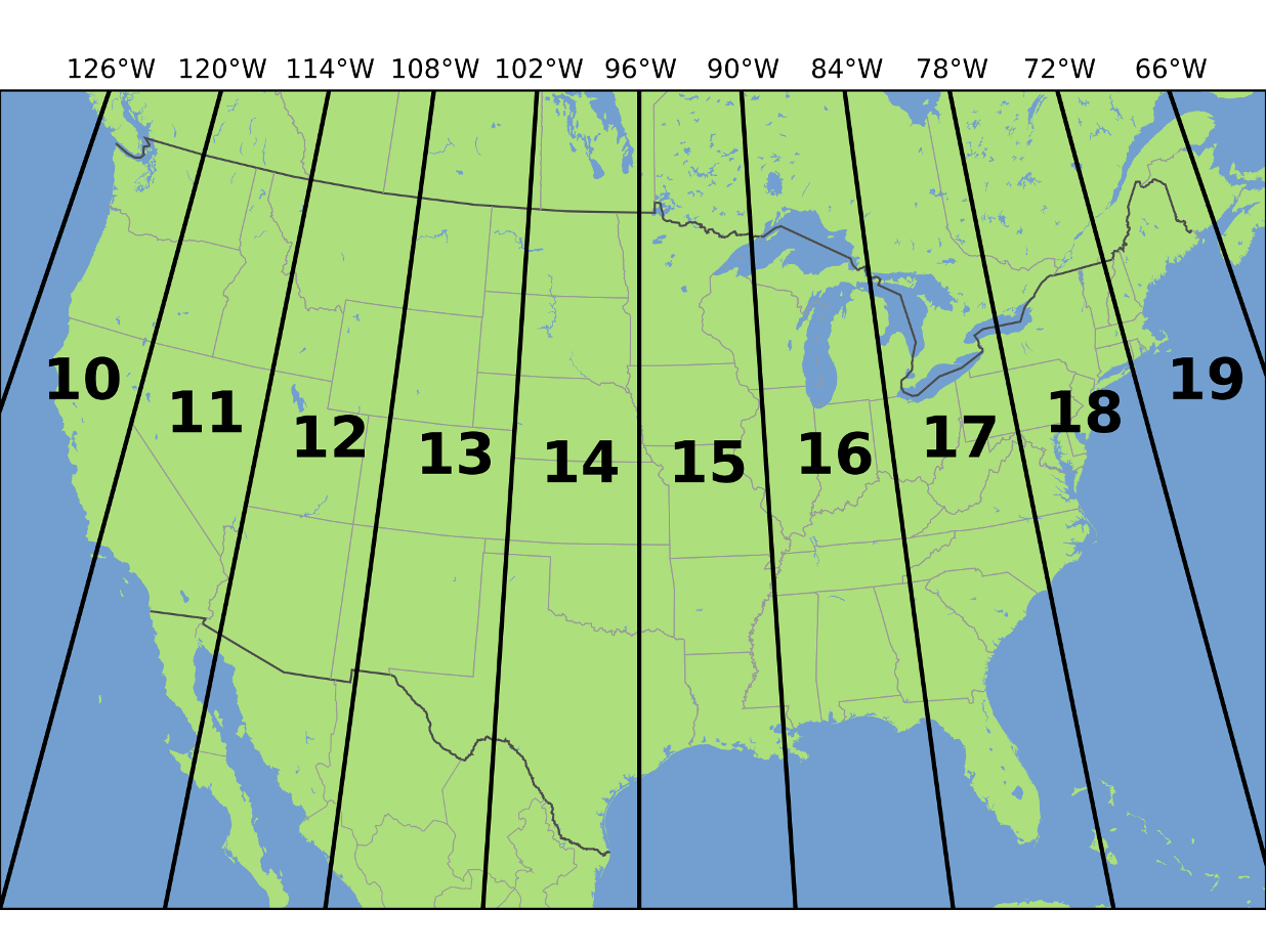
To measure area correctly, we must reproject data into a Projected Coordinate System (PCS) with linear units (i.e. meters). We can reproject a our data using the to_crs method.
counties_reproject = counties.to_crs('EPSG:32610')
counties_reproject.crs
<Projected CRS: EPSG:32610>
Name: WGS 84 / UTM zone 10N
Axis Info [cartesian]:
- E[east]: Easting (metre)
- N[north]: Northing (metre)
Area of Use:
- name: Between 126°W and 120°W, northern hemisphere between equator and 84°N, onshore and offshore. Canada - British Columbia (BC); Northwest Territories (NWT); Nunavut; Yukon. United States (USA) - Alaska (AK).
- bounds: (-126.0, 0.0, -120.0, 84.0)
Coordinate Operation:
- name: UTM zone 10N
- method: Transverse Mercator
Datum: World Geodetic System 1984 ensemble
- Ellipsoid: WGS 84
- Prime Meridian: Greenwich
Now our data has a projected CRS, we can calculate the area of each county with no warnings.
counties_reproject['area'] = counties_reproject['geometry'].area
counties_reproject.head()
| county | geometry | area | |
|---|---|---|---|
| 0 | Josephine County | POLYGON ((481194.491 4727816.88, 481194.958 47... | 4.246560e+09 |
| 1 | Curry County | POLYGON ((433625.945 4737685.67, 433625.841 47... | 5.162413e+09 |
| 2 | Jackson County | POLYGON ((558467.407 4760675.759, 558469.593 4... | 7.249715e+09 |
| 3 | Coos County | POLYGON ((433625.945 4737685.67, 433231.393 47... | 4.684074e+09 |
| 4 | Klamath County | POLYGON ((634511.459 4830645.879, 634517.742 4... | 1.588783e+10 |
counties_reproject.nlargest(n=10, columns='area')
| county | geometry | area | |
|---|---|---|---|
| 7 | Harney County | POLYGON ((882378.079 4887383.57, 882399.149 48... | 2.653973e+10 |
| 10 | Malheur County | POLYGON ((961062.868 4921620.315, 961060.411 4... | 2.581882e+10 |
| 5 | Lake County | POLYGON ((750439.186 4833367.767, 750479.131 4... | 2.165555e+10 |
| 4 | Klamath County | POLYGON ((634511.459 4830645.879, 634517.742 4... | 1.588783e+10 |
| 6 | Douglas County | POLYGON ((570239.73 4810068.418, 570239.824 48... | 1.328787e+10 |
| 8 | Lane County | POLYGON ((594233.362 4901694.354, 594237.353 4... | 1.222697e+10 |
| 15 | Grant County | POLYGON ((853221.257 4992269.09, 853253.647 49... | 1.174878e+10 |
| 33 | Umatilla County | POLYGON ((887375.271 5106291.097, 887517.231 5... | 8.385718e+09 |
| 32 | Wallowa County | POLYGON ((917855.824 5108106.858, 918248.122 5... | 8.197782e+09 |
| 19 | Baker County | POLYGON ((989277.799 5010475.028, 989270.732 5... | 8.026761e+09 |
More geometric properties#
There are other spatial methods we can apply to polygons such as the length of the outer edge (i.e. perimeter).
counties_reproject['perimeter'] = counties_reproject['geometry'].length
counties_reproject.head()
| county | geometry | area | perimeter | |
|---|---|---|---|---|
| 0 | Josephine County | POLYGON ((481194.491 4727816.88, 481194.958 47... | 4.246560e+09 | 331219.590167 |
| 1 | Curry County | POLYGON ((433625.945 4737685.67, 433625.841 47... | 5.162413e+09 | 438569.197122 |
| 2 | Jackson County | POLYGON ((558467.407 4760675.759, 558469.593 4... | 7.249715e+09 | 378774.026028 |
| 3 | Coos County | POLYGON ((433625.945 4737685.67, 433231.393 47... | 4.684074e+09 | 341177.939179 |
| 4 | Klamath County | POLYGON ((634511.459 4830645.879, 634517.742 4... | 1.588783e+10 | 619485.829095 |
Our cities GeoDataFrame also has geometric properties. We can access the latitude and longitude using the x and y methods.
cities['geometry'].x
0     -123.22
1     -118.56
2     -117.07
3     -123.10
4     -122.87
        ...
372   -122.42
373   -122.86
374   -124.10
375   -123.19
376   -123.29
Length: 377, dtype: float64
cities['geometry'].y
0      44.67
1      45.77
2      43.74
3      44.63
4      45.49
       ...
372    45.54
373    45.15
374    44.31
375    45.34
376    43.60
Length: 377, dtype: float64
Measure distance#
We can measure the distance between two points, provided they have a projected CRS.
cities_reproject = cities.to_crs('EPSG:32610')
eugene = cities_reproject[cities_reproject['name'] == 'Eugene'].reset_index()
bend = cities_reproject[cities_reproject['name'] == 'Bend'].reset_index()
eugene.distance(bend).values[0] / 1000
np.float64(144.97607871968486)
We can even compute the distance from Eugene to all cities in Oregon. We just have to convert our Eugene GeoDataFrame to a shapely Point object.
from shapely.geometry import Point
point = Point(eugene['geometry'].x, eugene['geometry'].y)
type(point)
shapely.geometry.point.Point
cities_reproject.distance(point)
0       68222.760516
1      407083.677355
2      487501.149310
3       63332.609637
4      160075.276651
           ...
372    173473.943528
373    122821.981564
374     83104.796535
375    142292.638317
376     52886.634459
Length: 377, dtype: float64
cities_reproject['dist_from_eugene'] = cities_reproject.distance(point) / 1000
cities_reproject.nsmallest(n=10, columns='dist_from_eugene')
| name | lat | lon | geometry | dist_from_eugene | |
|---|---|---|---|---|---|
| 100 | Eugene | 44.06 | -123.12 | POINT (490388.807 4878543.943) | 0.000000 |
| 62 | Coburg | 44.14 | -123.06 | POINT (495200.879 4887424.274) | 10.100312 |
| 309 | Springfield | 44.05 | -122.98 | POINT (501602.135 4877426.449) | 11.268874 |
| 74 | Creswell | 43.92 | -123.02 | POINT (498394.365 4862987.674) | 17.495327 |
| 346 | Veneta | 44.05 | -123.35 | POINT (471962.631 4877485.796) | 18.456534 |
| 166 | Junction City | 44.22 | -123.21 | POINT (483225.773 4896329.667) | 19.173968 |
| 139 | Harrisburg | 44.27 | -123.17 | POINT (486432.361 4901875.908) | 23.665038 |
| 69 | Cottage Grove | 43.80 | -123.06 | POINT (495173.424 4849661.421) | 29.276145 |
| 191 | Lowell | 43.92 | -122.78 | POINT (517661.989 4863011) | 31.386283 |
| 215 | Monroe | 44.32 | -123.30 | POINT (476077.414 4907459.292) | 32.263190 |
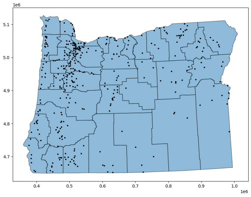
Plot#
If our data are in the same projection system, we can plot them together.
ax = counties_reproject.plot(figsize=(10, 10), alpha=0.5, edgecolor='k')
cities_reproject.plot(ax=ax, color='black', markersize=5)
<Axes: >
Spatial joins#
One of the most useful things about GeoPandas is that it contains functions to perform spatial joins to combine two GeoDataFrames based on the spatial relationships between their geometries.
The order of the two GeoDataFrames is quite important here, as well as the how argument. A left outer join implies that we are interested in retaining the geometries of the GeoDataFrame on the left, i.e. the point locations of the cities. We then retain attributes of the right GeoDataFrame if they intersect and drop them if they don’t.
The following would provide the county attributes for all our cities based on a spatial intersection.
cities_reproject.sjoin(counties_reproject, how="left").head()
| name | lat | lon | geometry | dist_from_eugene | index_right | county | area | perimeter | |
|---|---|---|---|---|---|---|---|---|---|
| 0 | Adair Village city | 44.67 | -123.22 | POINT (482561.392 4946316.184) | 68.222761 | 12 | Benton County | 1.755206e+09 | 235146.207283 |
| 1 | Adams | 45.77 | -118.56 | POINT (845212.127 5078087.252) | 407.083677 | 33 | Umatilla County | 8.385718e+09 | 481237.919385 |
| 2 | Adrian | 43.74 | -117.07 | POINT (977541.425 4860113.062) | 487.501149 | 10 | Malheur County | 2.581882e+10 | 768932.749866 |
| 3 | Albany | 44.63 | -123.10 | POINT (492067.91 4941854.29) | 63.332610 | 13 | Linn County | 5.969370e+09 | 426799.857671 |
| 4 | Aloha | 45.49 | -122.87 | POINT (510158.282 5037393.753) | 160.075277 | 27 | Washington County | 1.880526e+09 | 250776.514814 |
Note
The geometry column type is POINT.
On the other hand, a right outer join implies that we are interested in retaining the geometries of the GeoDataFrame on the right, i.e. the polygons of the counties. This time we keep all rows from the right GeoDataFrame and duplicate them if necessary to represent multiple hits between the two dataframes.
cities_reproject.sjoin(counties_reproject, how="right").head()
| index_left | name | lat | lon | dist_from_eugene | county | geometry | area | perimeter | |
|---|---|---|---|---|---|---|---|---|---|
| 0 | 53 | Cave Junction | 42.17 | -123.65 | 214.270534 | Josephine County | POLYGON ((481194.491 4727816.88, 481194.958 47... | 4.246560e+09 | 331219.590167 |
| 0 | 110 | Fruitdale | 42.42 | -123.30 | 182.712845 | Josephine County | POLYGON ((481194.491 4727816.88, 481194.958 47... | 4.246560e+09 | 331219.590167 |
| 0 | 128 | Grants Pass | 42.43 | -123.33 | 181.818198 | Josephine County | POLYGON ((481194.491 4727816.88, 481194.958 47... | 4.246560e+09 | 331219.590167 |
| 0 | 169 | Kerby | 42.20 | -123.65 | 211.006589 | Josephine County | POLYGON ((481194.491 4727816.88, 481194.958 47... | 4.246560e+09 | 331219.590167 |
| 0 | 203 | Merlin | 42.52 | -123.43 | 172.862986 | Josephine County | POLYGON ((481194.491 4727816.88, 481194.958 47... | 4.246560e+09 | 331219.590167 |
Which county contains the most cities/towns?#
We would do this would be to use the groupby function.
join = cities_reproject.sjoin(counties_reproject, how="left")
The first argument groupby accepts is the column we want group our data into (county in our case). Next, it takes a column (or list of columns) to summarize. Finally, this function does nothing until we specify how we want to group our data (count).
It’s actually nice to reset the index after using groupby so that we end up with a DataFrame (rather than a Series).
grouped = join.groupby('county')['name'].count().reset_index()
grouped.nlargest(n=10, columns='name')
| county | name | |
|---|---|---|
| 23 | Marion County | 25 |
| 33 | Washington County | 24 |
| 2 | Clackamas County | 23 |
| 9 | Douglas County | 23 |
| 21 | Linn County | 23 |
| 29 | Umatilla County | 19 |
| 28 | Tillamook County | 18 |
| 14 | Jackson County | 17 |
| 8 | Deschutes County | 14 |
| 19 | Lane County | 12 |
Which county is furthest from Eugene?#
grouped = join.groupby('county')['dist_from_eugene'].mean().reset_index()
grouped.nlargest(n=10, columns='dist_from_eugene')
| county | dist_from_eugene | |
|---|---|---|
| 31 | Wallowa County | 482.889501 |
| 22 | Malheur County | 470.534421 |
| 0 | Baker County | 440.425667 |
| 30 | Union County | 433.871378 |
| 29 | Umatilla County | 390.358136 |
| 12 | Harney County | 344.072705 |
| 11 | Grant County | 336.334826 |
| 24 | Morrow County | 324.247272 |
| 10 | Gilliam County | 281.414386 |
| 18 | Lake County | 280.863893 |